2026–27 Group & Individual Project III
Potential flows
Research area: Applied mathematics
⚠️ Individual Project III: I am on research leave in Epiphany, so some of our meetings in this term may take place by video call.
Overview
This is an applied mathematics project for students concurrently taking Fluid Mechanics III.
In general, fluids are complicated to model. Just like in Dynamics I, they still obey Newton’s second law, but the forces are complicated and the way we describe acceleration is also complicated!
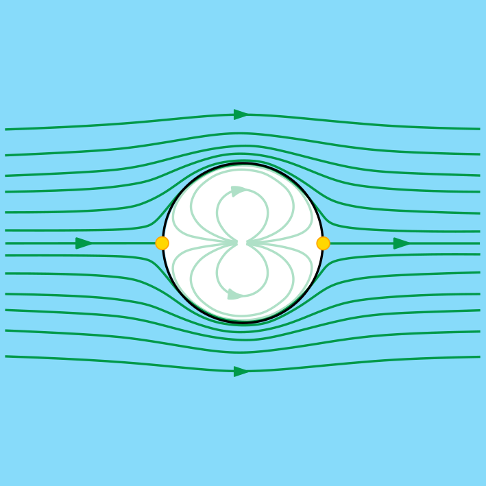
Thankfully though, there are some circumstances where the fluid’s velocity, $\boldsymbol{u}$, is easier to describe. Fluids that are, in the jargon, ‘incompressible, inviscid and irrotational’ – for example, smoothly flowing water with no vortices – can be described through their potential $\phi$, where $\boldsymbol{u}=\boldsymbol\nabla\phi$. And that potential obeys Laplace’s equation,
\[\nabla^2 \phi = 0.\]
In this project, we will solve this equation in a number of interesting ways and in a number of interesting domains.
We will do so primarily computationally, so you will learn how to code up a PDE solver in Python and perform numerical integration; but we can also use analytical methods like multipole expansions and conformal mapping to solve this equation in interesting domains.
We can then compare our methods, learning more about modelling and gaining an awareness of which tools are best for solving physical problems.
Corequisities
You will be taking Fluid Mechanics III at the same time. The fluids course will cover the basics of potential flow in the first weeks of term, but this project will go much deeper and give you an opportunity to apply the material you’ve learnt.
Prerequisites
This is an applied maths project where you will have to do some practical coding. You should therefore be confident in programming in Python.
Dynamics I, Complex Analysis II and Mathematical Methods II are essential. Computational Mathematics II is strongly recommended.
Group project
By the end of the group project we should be able to:
- define a potential flow,
- analytically derive its velocity in a set of nice geometries (e.g. flow around a cylinder),
- approximately derive its velocity in a not so nice geometry (e.g. flow around a cube or around a corner),
- implement and compare solvers for Laplace’s equation in Python in these geometries,
- quantify numerical accuracy (convergence, error),
- compare with experimental results in the literature.
Mode of operation and evidence of learning for the group project
The project will revolve around learning through reading and programming in Python. Students will demonstrate their understanding by comparing theory to simulations and experimental literature, writing Python code to implement core methodology, modelling a number of physically-inspired fluid flows, and clearly communicating the material in both written and oral formats.
Individual project
The individual project will build on the knowledge we have gained in the group project and will explore additional advanced topics. A few examples of topics you will be able to investigate are:
- presents an approximate analytic solution of the potential around a square: a lovely idea using multipoles. Would be nice to simulate as well using finite difference methods.
- Potential flows in a T-junction. Similar to stagnation point flows.
- Vortex interactions
- Weird shapes using conformal maps
- What about convergence?
- Represent flow using distributions on complex boundaries (e.g. Katz & Plotkin §3.14)
- Slender body theory (e.g. Katz & Plotkin §8.3)
- Matching potential flow to boundary layers (e.g. Katz & Plotkin §14)
Mode of operation and evidence of learning for the individual project
The project will revolve around learning through reading and programming in Python. Students will demonstrate their understanding by comparing theory to simulations and experimental literature, writing Python code to implement core methodology, modelling a number of physically-inspired fluid flows, and clearly communicating the material in both written and oral formats.